Technical Report · Retail Replenishment
Better Forecasts or Better Inventory Decisions: What Creates More Value?
Measuring the financial value of better forecasts and inventory decisions through a reproducible study of three forecasting methods and three planning policies, using real fresh-retail sales across 30 stores, 40 products, and five weeks—with every result expressed in monetary terms.
$7.8M
A year, per $1B of sales, from planning the stores as one network instead of one shelf at a time (illustrative).
$1.7M
What a slightly better forecast is worth a year: real, but a fraction of the network plan’s gain.
−32%
Leftover stock when the distribution center (DC) runs short, at a higher fill rate.
$10.8M
What a poor forecast costs a year: more than the network plan recovers.
TLDR: Once you have a reasonably good sales forecast, deciding where to put your stock can create more value than making the forecast slightly more accurate. For example, moving extra products from a store with too much stock to one that’s running out can reduce waste and prevent lost sales. The conclusion: better predictions help, but what you do with them matters just as much.
Data: FreshRetailNet-50K, Dingdong-Inc, CC BY 4.0. Sales are normalized, so dollar figures are illustrative: $1B a year of sales at a 30% gross margin. Every number traces to a Harumi run (Section 8). Select any figure, table or formula to open the full-size image.
At a glance
THE QUESTION
Every replenishment team debates its forecast. Fewer debate the decision made with it. When the DC cannot cover every store, and some stores hold stock that others need, how much is a better forecast worth, and how much is a better decision worth? We put both in money.
WHAT WE DID
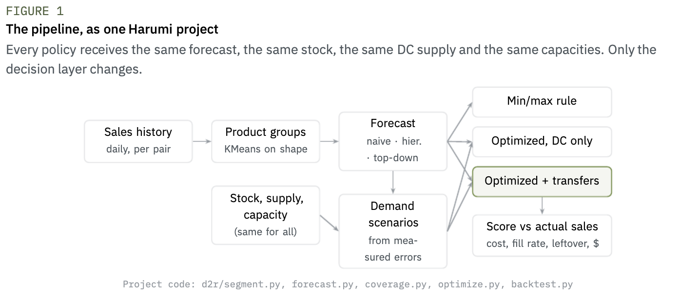
• Built the full pipeline as one Harumi project: product grouping, three forecasts, the min/max rule most retailers run, and an optimization model that can also move stock between stores.
• Backtested every combination on 5 weeks of real sales from 30 stores and 40 fresh products, under a tight DC (60% of what stores need) and an ample one (130%).
• Scored each plan against the sales that actually happened, and translated the cost into dollars for a reference retailer with $1B a year of sales.
WHAT WE FOUND
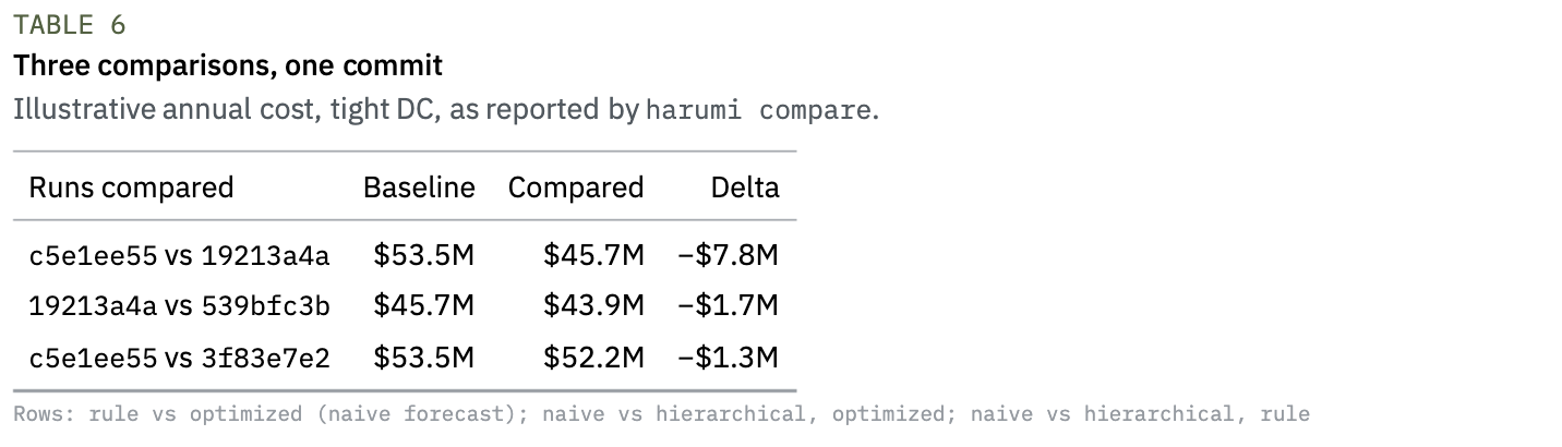
• The network decision is worth the most. With a tight DC, letting the plan move stock between stores lowered cost by 14.5%, cut leftover stock by 32.0% and raised the fill rate from 94.1% to 94.7%: about $7.8M a year per $1B of sales, of which $5.5M is sales the rule would have lost.
• Optimizing DC shipments alone barely beat a good rule: −1.1% cost, worth $584.8k a year.
• A better forecast is worth real money, but less. A forecast 0.3 points more accurate was worth $1.3M to $1.7M a year.
• A poor forecast costs more than optimization recovers. The classic top-down split cost $9.1M to $10.8M a year more than the naive forecast. With it, even the network plan did worse than the plain rule on the naive forecast.
WHAT IT MEANS FOR YOUR OPERATION
• Get the forecast roughly right, then put the effort into the decision made with it.
• Price a forecast upgrade before you pay for it, or before you dismiss it.
• Treat trade-offs, such as service against leftover stock, as business inputs you set, not as solver outputs.
WHAT THIS DOES NOT SHOW
The source sales are normalized and the stock positions are synthetic, so dollar figures are illustrative and the size of the transfer gain depends on how unbalanced the network is. Section 7 lists every limit.
HOW TO READ THIS REPORT
Sections 1 and 2 set up the question and the experiment. Sections 3 and 4 give the forecasting methods, the scenario generation and the full optimization model, for operations research readers. Sections 5 to 7 hold the results, what they mean and what they do not support. Section 8 lists the Harumi runs behind every number.
01. The question
Retail replenishment has two layers. A forecast estimates how much each store will sell of each product. A decision turns that estimate into stock: how much the distribution center ships to each store, and whether any store should send stock to another. Most of the effort, and most of the debate, goes into the first layer.
The second layer is often a min/max rule: when a store’s stock covers fewer than a minimum number of days of forecast demand, order up to a maximum number of days. The rule is simple, explainable and local. It decides each store and product on its own. It cannot see that one store holds stock another store needs, and when the DC runs short, it can only cut every order in the same proportion.
We wanted to know which layer is worth more, and by how much, in money. So we built both into one Harumi project and ran a factorial experiment on public fresh-retail data: three forecasts, three planning policies and two DC supply levels, all from the same code, every plan scored against the sales that actually happened.
1.1 What this report contributes
• A priced comparison of the two layers on the same data, the same stock and the same supply, so the difference between two runs comes from one change only.
• A two-stage stochastic model for weekly replenishment with store-to-store transfers, with a fixed cost per route, solved by an LP-guided two-phase method that reports its distance to a lower bound of the full model (at most 3.1% here).
• A comparison that does not depend on the cost weights: service against leftover stock, across settings of the rule and of the model.
• A money translation computed inside the run, so every dollar figure has a stated basis.
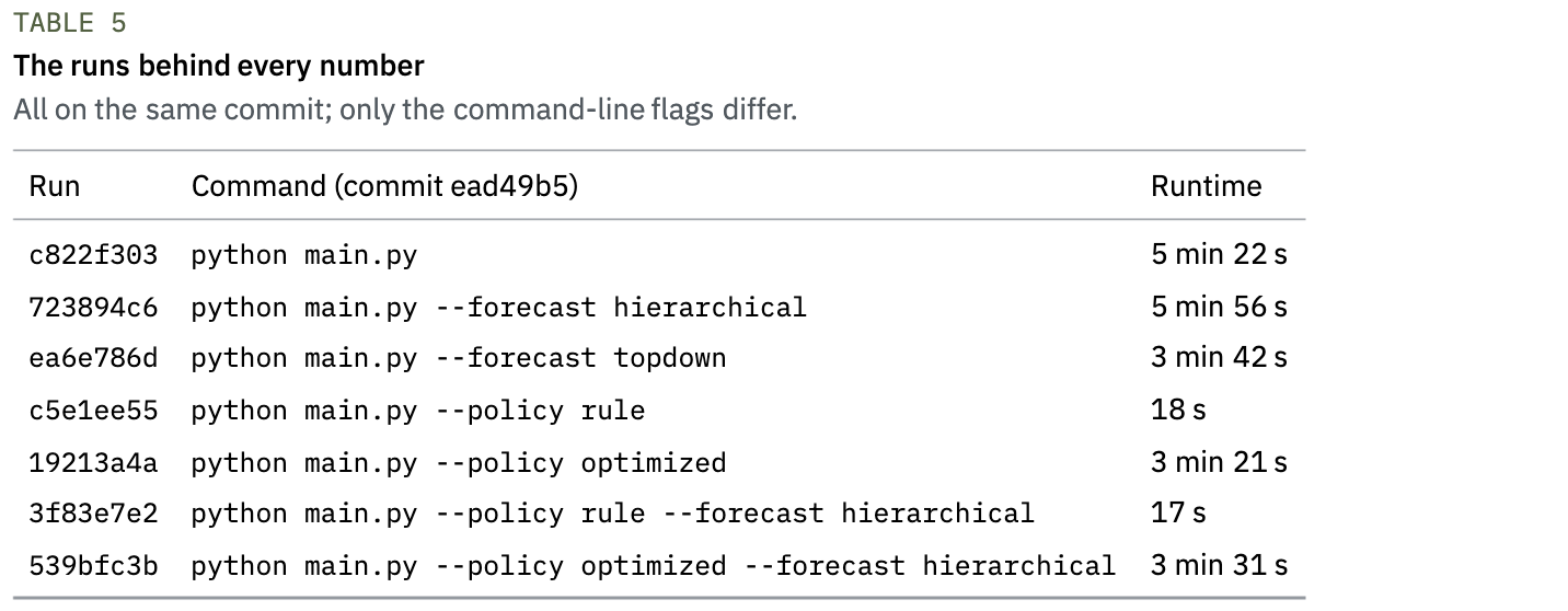
• Full reproducibility: 7 Harumi runs on one commit, compared with harumi compare.
1.2 Related work
Moving stock between locations at the same echelon is known as lateral transshipment. Paterson et al. (2011) review the literature and separate reactive transshipments, used to meet demand that stock on hand cannot satisfy, from proactive ones, made at predetermined moments to redistribute stock. Our model is proactive: transfers and DC shipments are decided together at the start of each week. Planning against a set of sampled demand scenarios is the sample average approximation of a two-stage stochastic program (Birge and Louveaux, 2011; Kleywegt et al., 2002). On the forecasting side, splitting a group forecast by historical shares is the classic top-down method (Gross and Sohl, 1990), and the seasonal naive forecast is the standard benchmark that any method should beat (Hyndman and Athanasopoulos, 2021). The data come from FreshRetailNet-50K (Wang et al., 2025).
02. Data and experimental design
2.1 Data
FreshRetailNet-50K is a public benchmark released by Dingdong under a CC BY 4.0 license. It holds 50,000 hourly store-product sales series from 898 stores in 18 cities, covering 863 perishable products, with stockout periods annotated (Wang et al., 2025). We use the daily sales of one city: 40 products in 30 stores, the 1,166 store-product pairs with sales history, over 97 days (2024-03-28 to 2024-07-02). The publisher normalizes sales, so quantities in this report are relative units and costs are relative weights.
2.2 What we had to assume
The dataset has sales but no inventory, so four inputs are synthetic and held fixed across every policy and forecast:
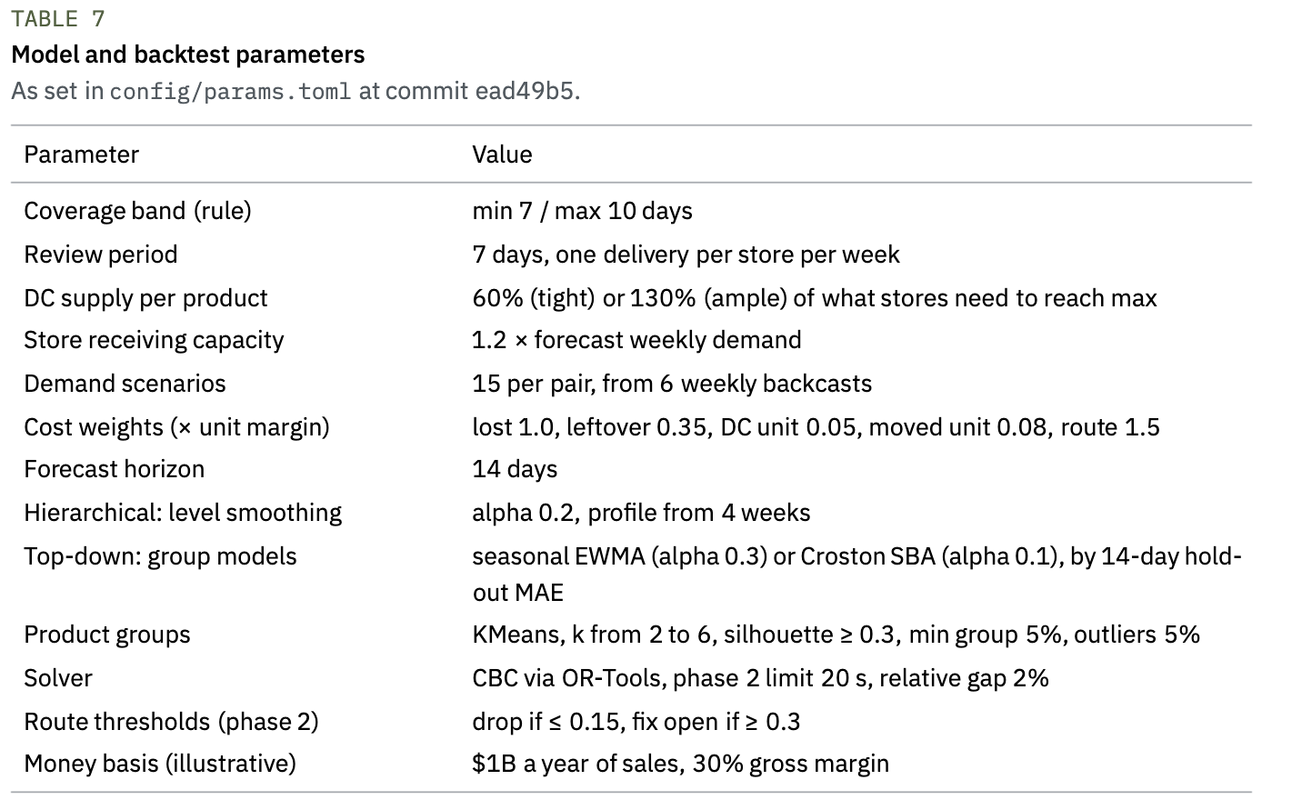
• Stock at each weekly snapshot: uniform between 0 and 14 days of each pair’s recent sales, seeded. The network is unbalanced on purpose, as real networks often are.
• Coverage band for the rule: minimum 7, maximum 10 days, for every store.
• DC supply per product: 60% (tight) or 130% (ample) of what the stores need to reach their maximum coverage.
• Store receiving capacity: 1.2 times the store’s forecast weekly demand.
2.3 Backtest protocol
The backtest uses a rolling origin, one origin per week, from 2024-05-29 to 2024-06-26. At each origin, using only data before it, the pipeline:
1. groups products by the shape of their demand;
2. forecasts the next 14 days for every pair with the plan’s forecast, and measures all three methods;
3. measures the plan’s forecast on the 6 previous weeks and turns those errors into demand scenarios;
4. plans the week with each policy, under each supply level;
5. scores each plan against the sales recorded in the 7 days that follow.
There is one delivery per store per week, at the start of the week. Demand that is not served is lost, and stock left at the end of the week counts as leftover, which for fresh products is mostly waste. Each week starts from its own stock snapshot, so a policy’s leftover does not carry into the next week.
2.4 Experimental design
The design is full factorial: 3 forecasts × 3 policies × 2 supply levels, each cell over the same 5 weeks. Within a forecast and a supply level, the three policies see identical inputs, so their comparison is paired. Each forecast is a separate Harumi run of the same commit (ead49b5); 4 further single-policy runs feed harumi compare (Section 8).
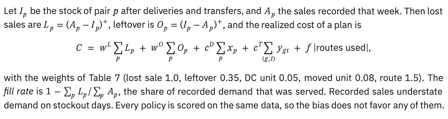
2.5 How a plan is scored
03. Forecasts and demand scenarios
3.1 Product groups
Sparse series forecast poorly on their own, so products borrow strength from similar ones. For each product, summed over stores, we compute eleven shape features of the daily series: coefficient of variation, peak-to-mean ratio, share of days with sales, mean and variation of the gaps between sales, temporal entropy, autocorrelation at lags 1 and 7, day-of-week strength, low-frequency spectral share and the 28-day trend. Features are standardized and clustered with KMeans, with k between 2 and 6 chosen by the silhouette score (Rousseeuw, 1987) (at least 0.3, no group under 5% of products). Products that look like no one else, flagged by an isolation forest (Liu et al., 2008) or lying far from every centroid, go to an OTHER group. In the latest week the method found k = 2 groups (silhouette 0.51) and 2 products in OTHER.
3.2 Three forecasts
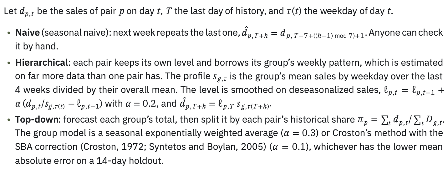
The plan uses the naive forecast. Every run measures all three, and a command-line flag (--forecast) switches the plan’s forecast, which is how the forecast study in Section 5 was run.
3.3 How accuracy is measured
Accuracy is the weighted absolute percentage error (WAPE) of weekly totals per store and product,

pooled over the weeks measured. Simply put, it is the share of the week’s sales that the forecast missed, counting misses in both directions. We report it on the 5 backtest weeks and on the 6 weeks before each origin.
3.4 Demand scenarios from the forecast's own errors

each scenario equally likely. In practice, the spread of the scenarios is the spread of the forecast’s past errors. A worse forecast produces wider scenarios, and the model hedges more.
04. Planning policies
4.1 The min/max rule (baseline)

4.2 The optimization model
The model decides, for one week and all products at once, what the DC ships to each pair and what each store sends to another, so as to minimize the expected cost over the demand scenarios.
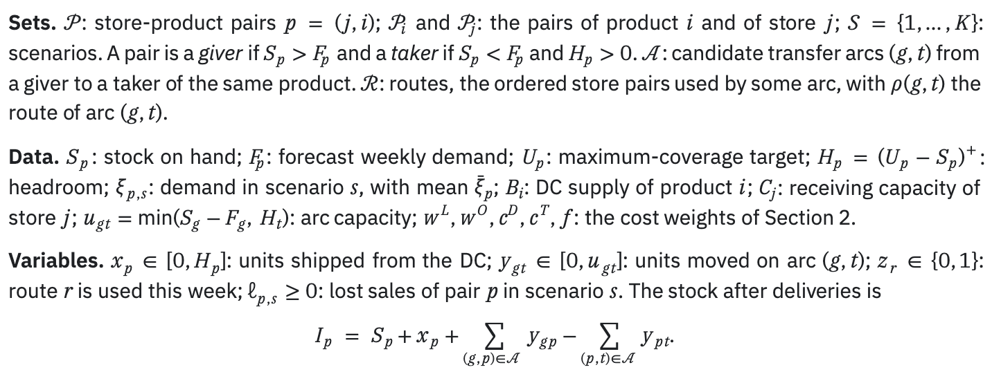
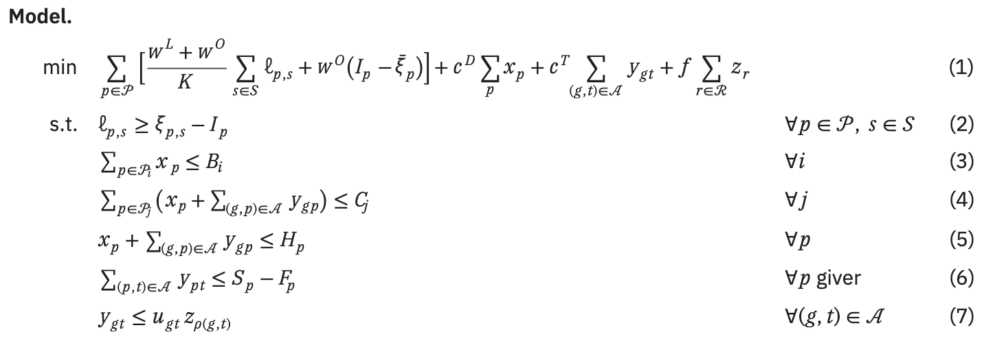
Constraint (3) is the DC’s supply, (4) each store’s receiving capacity, (5) the maximum coverage, and (6) keeps a giver’s own forecast week of stock. Two modeling choices matter:

• Linking per arc, not per route. Constraint (7) could be written once per route with a big M. Writing it once per arc adds rows but gives a much tighter LP relaxation, the classic strong formulation of fixed-charge flows. That tightness is what lets the method below close in seconds.
Removing y and z gives the DC-only policy, a linear program.
4.3 Solution method and its certificate
The fixed cost per route makes the problem a mixed-integer program. We solve it in two phases with CBC (Forrest and Lougee-Heimer, 2005) through OR-Tools (https://developers.google.com/optimization):
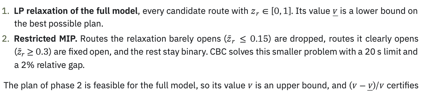
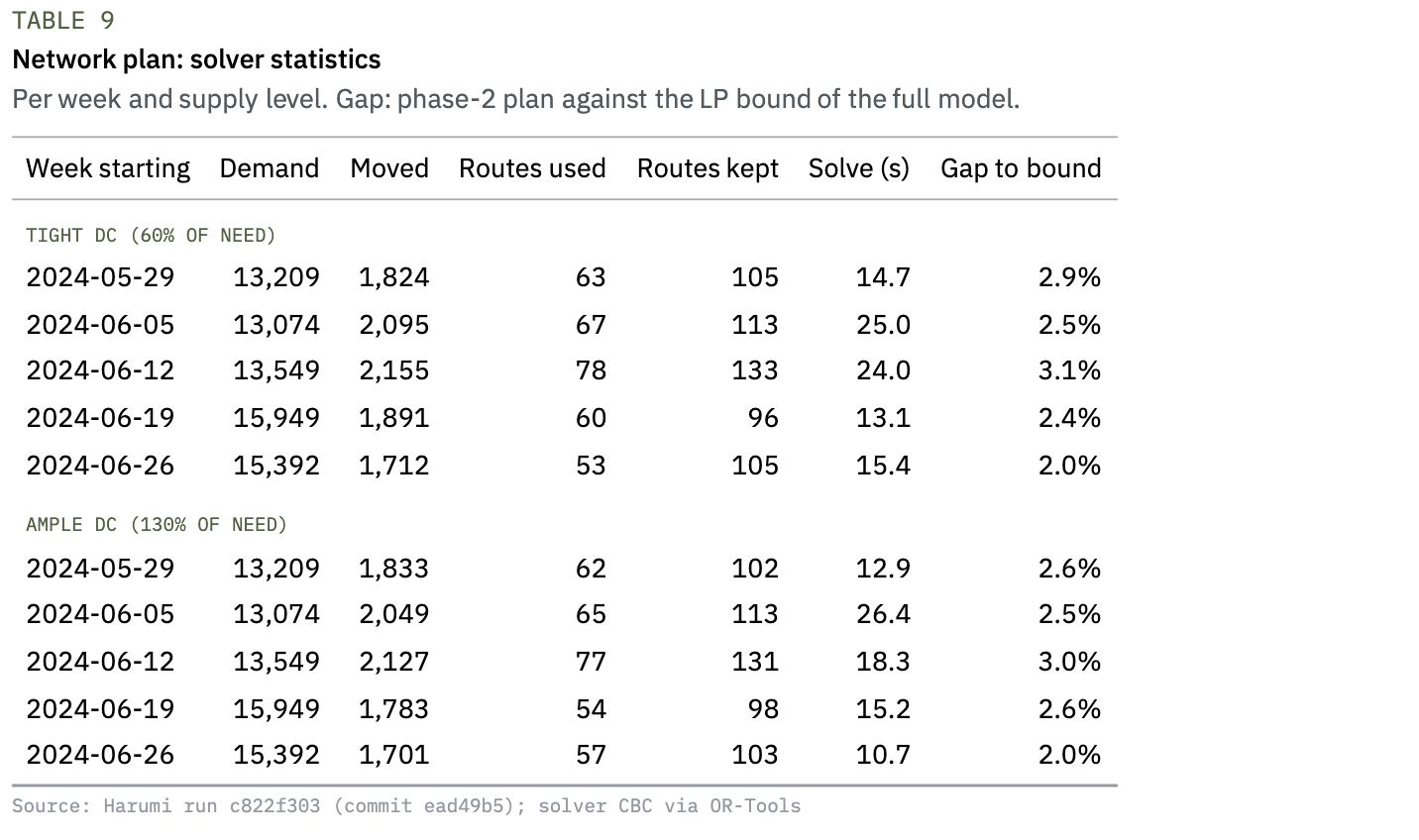
how far it can be from the best plan over all routes, not only the kept ones. Across the 10 week and supply combinations, 870 candidate routes (every ordered pair of stores) were reduced to 96–133, each solve took 10.7 s to 26.4 s, and the certified gap was 2.0% to 3.1% (Table 9). The DC-only linear program solved in at most 0.11 s.
05. Results
5.1 Same forecast, three decisions
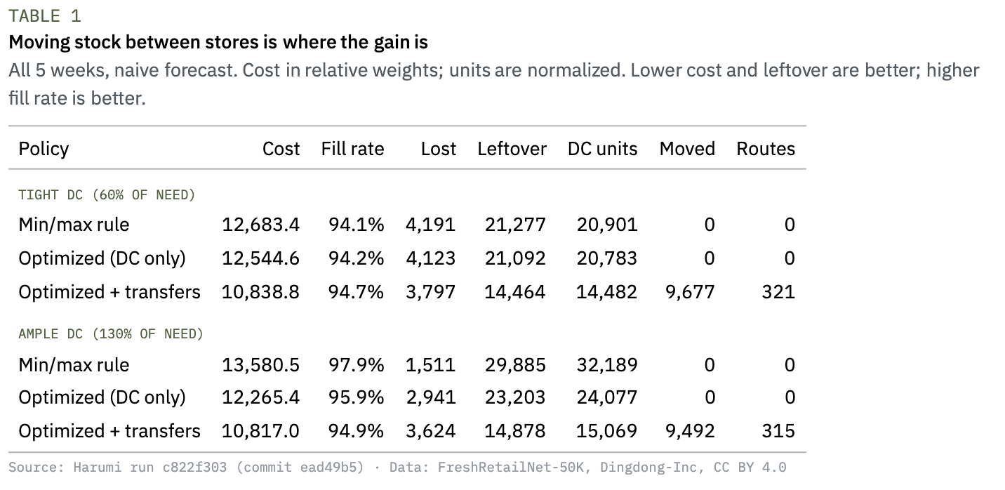
Table 1 compares the three policies on the naive forecast, summed over the 5 weeks.
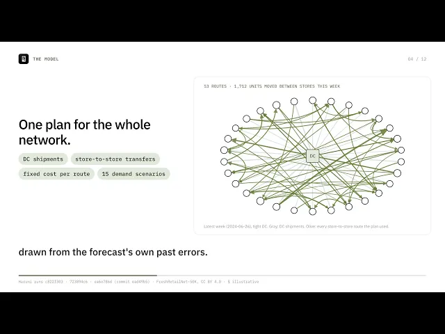
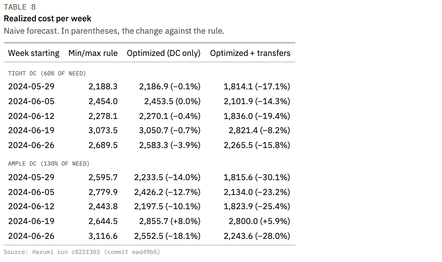
Tight DC. Optimizing DC shipments alone changed cost by −1.1% and the fill rate by +0.1 pts. On shipments alone, a well-tuned rule leaves little on the table: when the DC is short, the only lever is who gets the scarce units, and a pro-rata cut is a reasonable answer. Allowing transfers changed the picture: cost −14.5%, fill rate +0.6 pts and leftover −32.0%. The network plan moved 1,935 units a week on 64 routes, about 14% of weekly sales, and shipped less from the DC, because part of the need was met with stock already in the network.
Ample DC. With more supply than the stores need, both optimized policies cut cost by trading service for less leftover: the network plan lowered cost by 20.3% with 50.2% less leftover, but its fill rate was 3.0 pts below the rule’s 97.9%. That trade is set by the leftover weight, so Section 5.2 compares the policies at equal service instead.
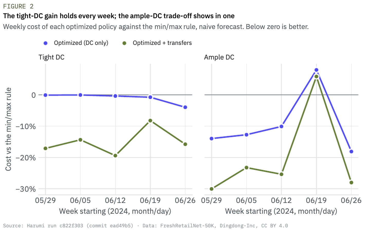
Week by week. Figure 2 shows each week on its own. With a tight DC, the network plan cost less than the rule in 5 of 5 weeks, by 8% to 19%. With an ample DC it cost less in 4 of 5. The exception is the week of 2024-06-19, when demand rose 18% over the week before. The rule’s larger buffers absorbed more of the jump: it lost 818 units of sales against 1,744 for the network plan, and both optimized plans cost more than the rule that week (+8% DC only, +6% with transfers). With 5 weeks, an exact two-sided sign test on the weekly wins gives p = 0.06 for the tight DC and p = 0.38 for the ample one. The count of wins alone cannot rule out chance; the size and consistency of the tight-DC gap carry the evidence.
5.2 Service against leftover, without cost weights
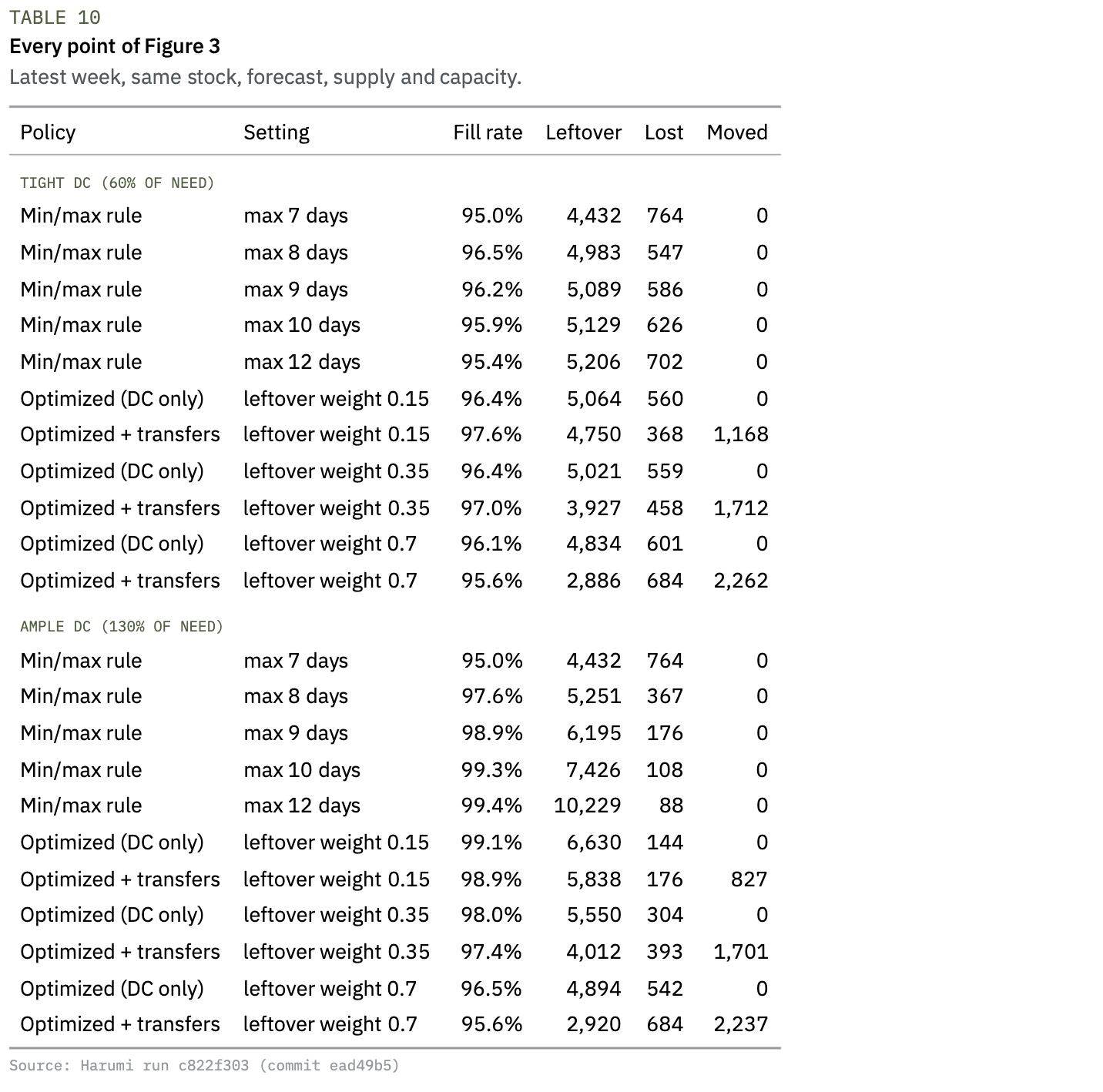
Any cost comparison depends on the weights. To remove them, in the latest week (2024-06-26) we ran the rule at every maximum coverage from 7 to 12 days and the model at three leftover weights (0.15, 0.35, 0.7), with the same stock, forecast, supply and capacity, and plotted fill rate against leftover (Figure 3). Up and to the left is better on both counts.
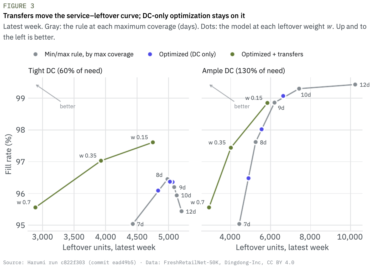
Three observations:
• The DC-only model lands on the rule’s curve. At the rule’s fill rate, its leftover differs from the rule’s by +0.1% (tight DC, w = 0.35) and −0.2% (ample). Without transfers, the model mostly picks a different point on the same curve.
• The network plan moves the curve. With a tight DC, at w = 0.35 it reached 97.0% fill with 3,927 units of leftover. Every rule setting did worse on both counts: the best rule fill rate was 96.5% and the lowest rule leftover was 4,432. With an ample DC, at equal fill rate, it carried 5.7%, 22.8% and 36.5% less leftover than the rule at w = 0.15, 0.35 and 0.7.
• With a tight DC, a higher target does not help the rule. The rule’s fill rate peaks at 8 days and falls beyond it. With supply fixed, a higher target cannot add stock; it only changes how the pro-rata cut spreads it.
5.3 Three forecasts, priced through the plan
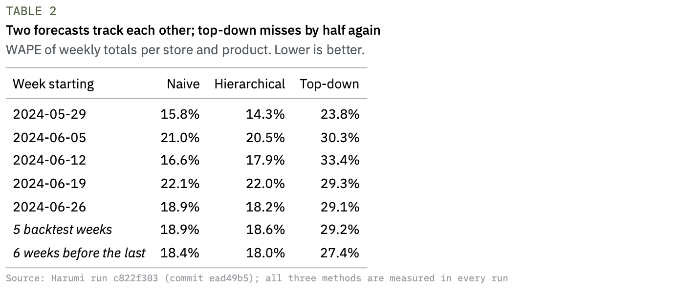
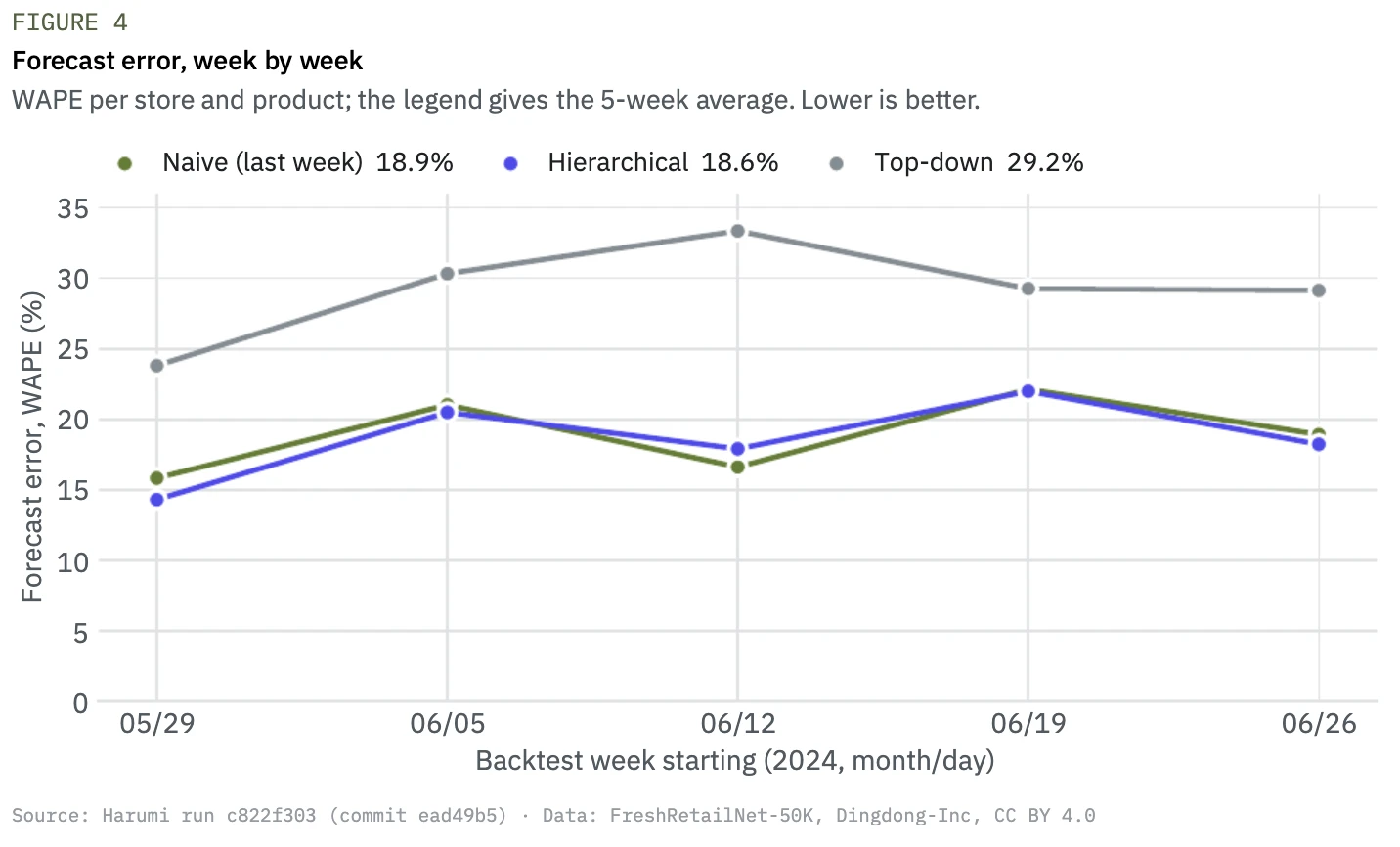
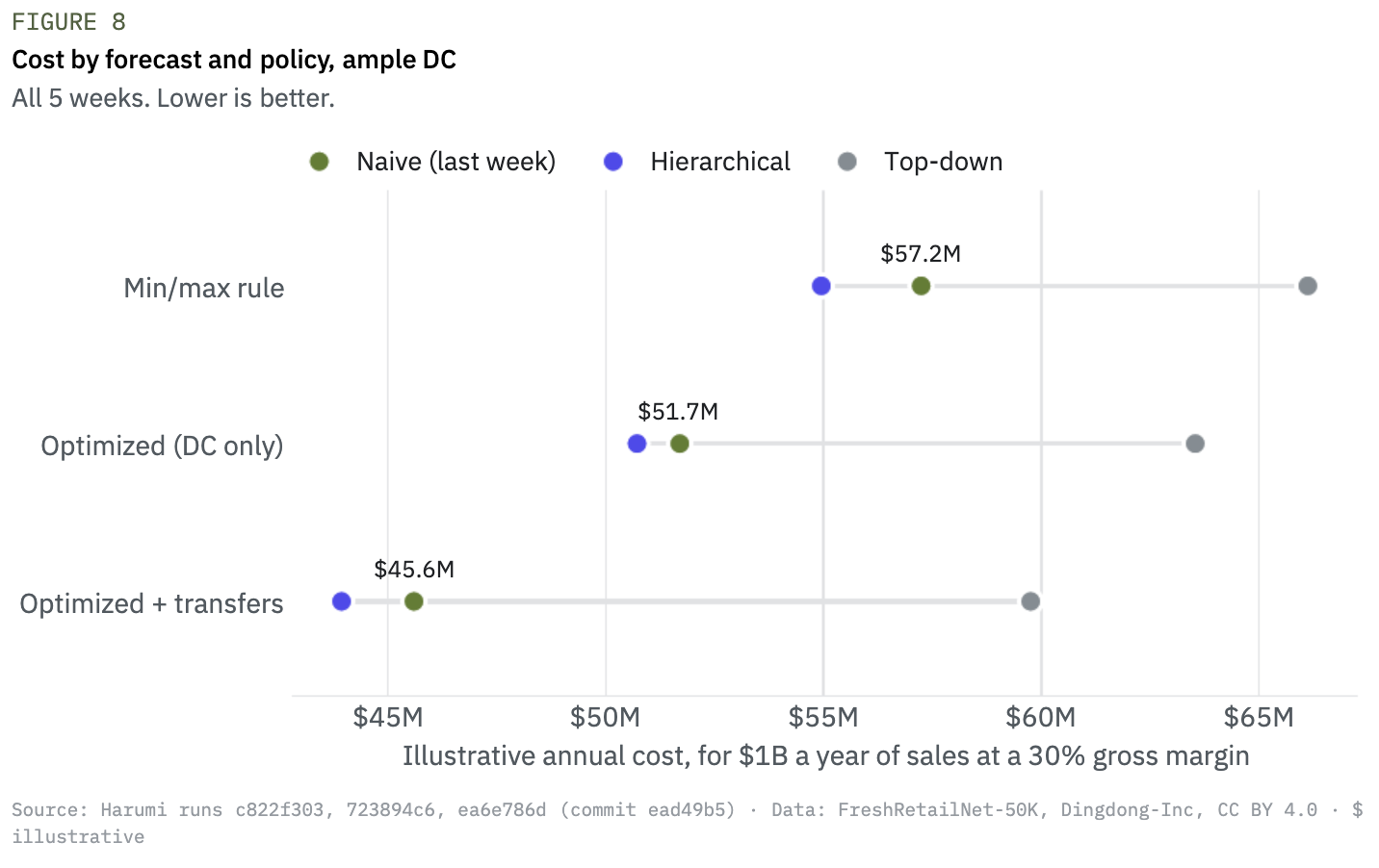
Table 2 gives the accuracy of the three forecasts and Figure 4 shows it week by week. Naive and hierarchical track each other within 0.3 points; top-down misses by 10.3 points more than naive, and it also lost in the 6 weeks before the backtest.
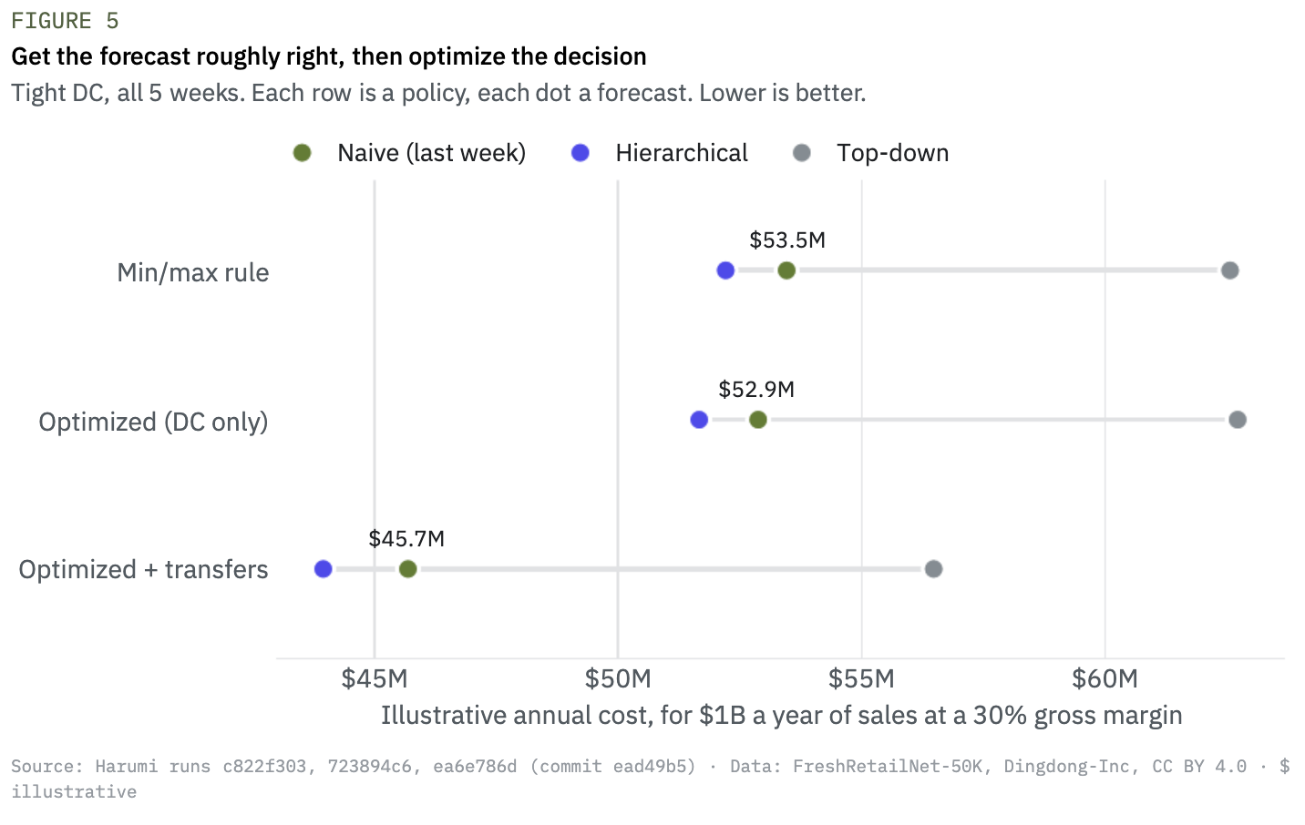
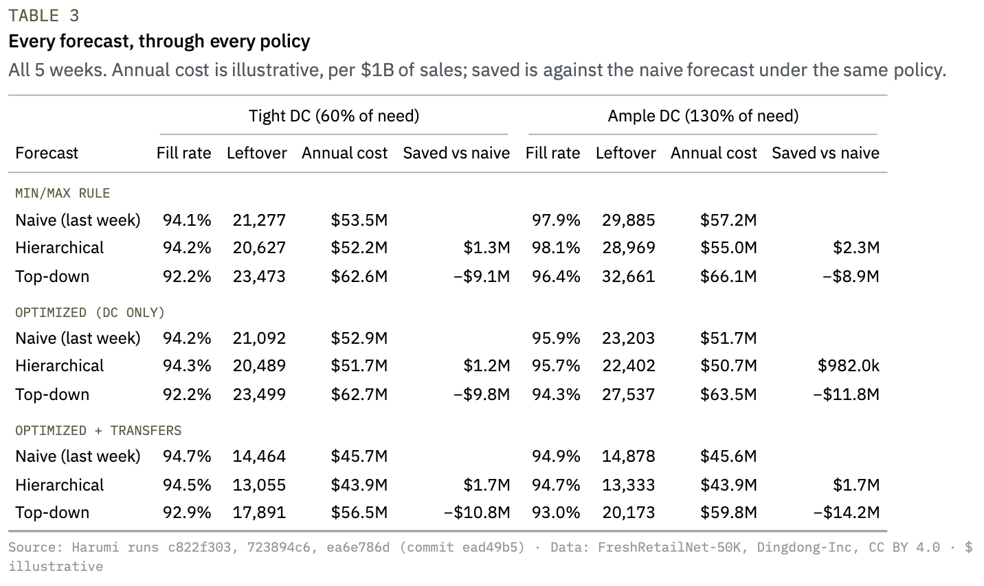
An error metric does not say what a forecast is worth. So we re-ran the whole backtest once per forecast, same commit, same data, only the --forecast flag changed, and priced each plan (Figure 5, Table 3). With a tight DC:
• The better forecast was worth $1.3M to $1.7M a year (rule and network plan), for a 0.3-point gain in WAPE.
• The poor forecast cost $9.1M to $10.8M a year more than naive. With it, even the network plan ($56.5M) did worse than the plain rule on the naive forecast ($53.5M).
• Forecast and decision are complements. The network plan was worth $7.8M over the rule with the naive forecast, $8.3M with the hierarchical one and only $6.1M with top-down. A poor forecast shrinks what the decision can recover.
5.4 What it is worth in money
The source data is normalized, so dollars cannot be measured; they can only be translated, and the translation is part of the run. We read the cost weights as multiples of one unit’s gross margin: a lost sale loses its margin (weight 1.0), a leftover unit costs 0.35 of it. For a reference retailer with annual sales R in these categories at gross margin m, a policy with realized cost C on demand D costs

taking the backtest weeks as representative of the year. Here R is $1B and m is 30%, both set in the project’s parameters, so any retailer can put its own numbers in and re-run.
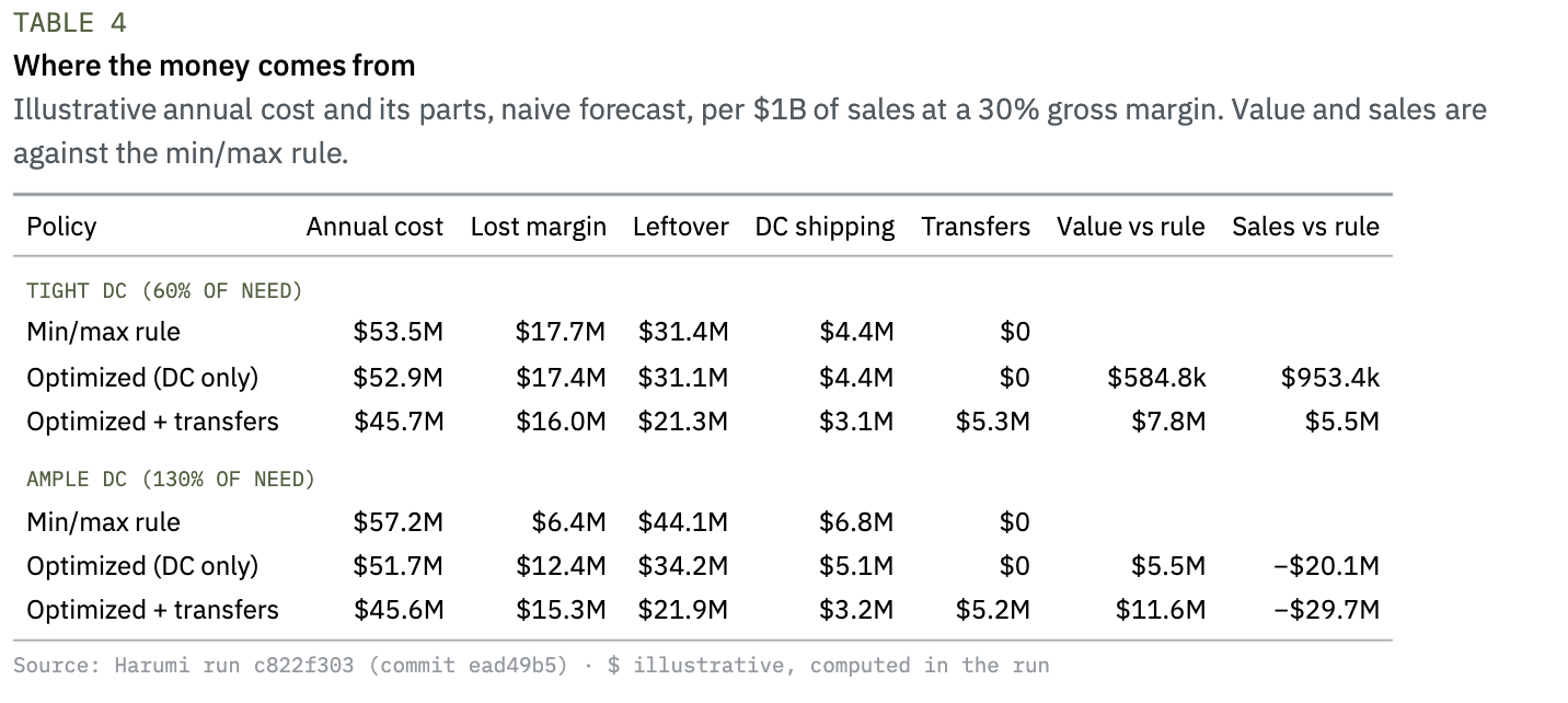
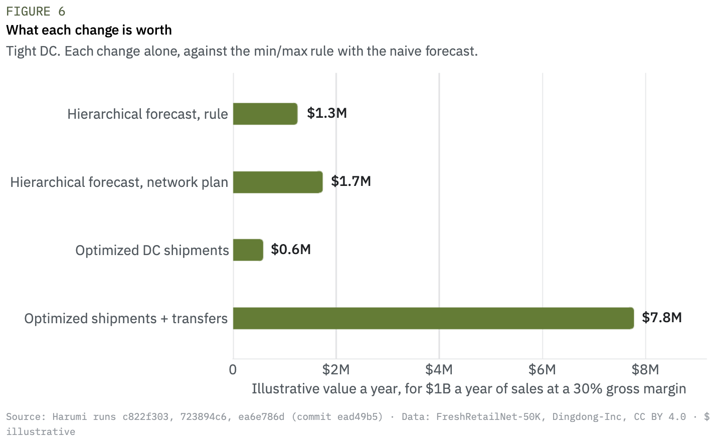
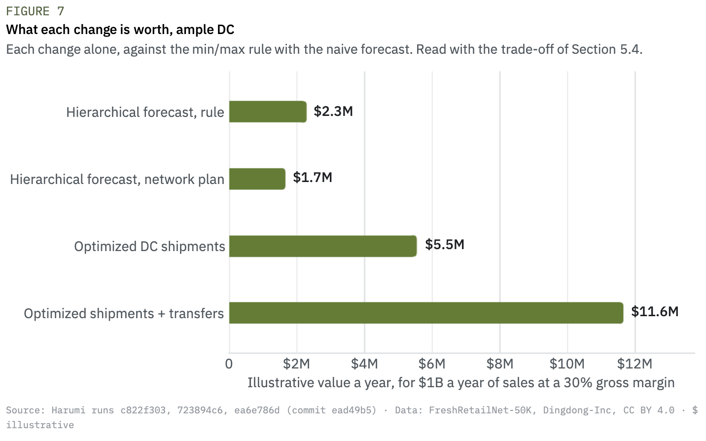
With a tight DC, the network plan is worth $7.8M a year (Table 4). It spends $5.3M a year on transfers to save $10.1M of leftover, $1.4M of DC shipping and $1.7M of lost margin, and it recovers $5.5M of sales. Figure 6 puts each change side by side.
The ample-DC trade-off, in plain sight. With an ample DC, the network plan lowers the illustrative cost by $11.6M a year, but it gives up $29.7M of sales to do it. Whether that is a good trade depends on what a leftover unit of fresh product really costs. That is a business input, not a solver output, so the project exposes it as a parameter, and the equal-service comparison of Section 5.2 shows the result does not hinge on it.
06. What it means
Get the forecast roughly right, then optimize the decision. A poor forecast costs more than optimization can recover. Between two reasonable forecasts, the difference is real but smaller, and the network decision is worth several times more.
The decision layer is where the network is. A rule, or a model limited to the same levers, decides each shelf on its own. The gain came from the lever a rule does not have: using stock already in the network.
Simplicity has a price, and now it has a number. We plan with the naive forecast because every planner can check it by hand. That choice costs about $1.7M a year per $1B of sales on this data. Simplicity and trust on one side, a priced gain on the other: the retailer decides, and the decision can be revisited each week because all three forecasts stay measured.
Trade-offs are parameters. The ample-DC result stands or falls with the cost of a leftover unit. Making that cost an explicit input, and showing the service–leftover curve, turns a debate about the solver into a business choice.
FOR OPERATIONS LEADERS
Before you invest in a better forecast or a new planning tool, price both on your own data: run the current rule, the candidate and the alternatives on the same weeks, the same stock and the same supply, and compare the cost in money. That is a few runs on Harumi, not a project.
07. What this does not show
• The dollar figures are illustrative. Sales in the source are normalized. Dollars come from two stated assumptions, annual sales and gross margin, plus the cost weights. None is a measured saving.
• The stock positions are synthetic and deliberately unbalanced, which is what makes transfers pay off. The network plan moved 1,935 units a week, about 14% of sales. That is a lot of store-to-store traffic for a real operation, and a real deployment would cap it.
• Recorded sales understate demand on stockout days. The dataset annotates stockouts and its authors recover latent demand from them (Wang et al., 2025); this study does not yet use that.
• Each week stands alone. Stock does not carry over between weeks, deliveries arrive at the start of the week, and shelf life is priced through the leftover weight rather than modeled.
• 5 weeks, 1 city, 40 products. Enough to compare methods on identical inputs, not to promise an outcome. A sign test on 5 weeks cannot reach conventional significance by itself.
• The model’s plans are within 3.1% of the lower bound of the full model, measured on the in-sample scenarios. The realized costs reported here are out of sample: they come from the actual sales.
• The coverage band, DC supply, receiving capacity and cost weights are assumptions (Table 7). Your numbers come from your data.
08. Reproducibility on Harumi
The whole study is one git repository on Harumi: data preparation, product grouping, three forecasts, the rule, the OR-Tools model, the backtest and three dashboards. A full run takes 5 min 22 s on the or_python_medium kernel. The key performance indicators (cost, fill rate, leftover and the illustrative annual cost), their direction and the primary one are declared in the project’s configuration, so every run is scored the same way.
harumi compare puts two runs side by side, KPI by KPI. Table 6 shows the illustrative annual cost with a tight DC for the three comparisons used here: rule against optimization, and naive against hierarchical forecast under each policy.
Every number in this report is generated from these runs by a script; none is typed by hand.
PRICE YOUR OWN FORECAST AND DECISIONS
If you want to know what your forecast and your replenishment decisions are worth on your own data, that is the conversation we like to have. Book a demo at harumi.io.
A. Parameters
B. Week by week
C. Service against leftover, latest week
D. Ample DC
References
Birge, J. R. and Louveaux, F. (2011). Introduction to Stochastic Programming, 2nd ed. Springer.
Croston, J. D. (1972). Forecasting and stock control for intermittent demands. Operational Research Quarterly, 23(3), 289–303.
Forrest, J. and Lougee-Heimer, R. (2005). CBC user guide. In Tutorials in Operations Research: Emerging Theory, Methods, and Applications. INFORMS.
Gross, C. W. and Sohl, J. E. (1990). Disaggregation methods to expedite product line forecasting. Journal of Forecasting, 9(3), 233–254.
Hyndman, R. J. and Athanasopoulos, G. (2021). Forecasting: Principles and Practice, 3rd ed. OTexts.
Kleywegt, A. J., Shapiro, A. and Homem-de-Mello, T. (2002). The sample average approximation method for stochastic discrete optimization. SIAM Journal on Optimization, 12(2), 479–502.
Liu, F. T., Ting, K. M. and Zhou, Z.-H. (2008). Isolation forest. In Proceedings of the 8th IEEE International Conference on Data Mining, 413–422.
Paterson, C., Kiesmüller, G., Teunter, R. and Glazebrook, K. (2011). Inventory models with lateral transshipments: a review. European Journal of Operational Research, 210(2), 125–136.
Rousseeuw, P. J. (1987). Silhouettes: a graphical aid to the interpretation and validation of cluster analysis. Journal of Computational and Applied Mathematics, 20, 53–65.
Syntetos, A. A. and Boylan, J. E. (2005). The accuracy of intermittent demand estimates. International Journal of Forecasting, 21(2), 303–314.
Wang, Y., Gu, J., Long, L., Li, X., Shen, L., Fu, Z., Zhou, X. and Jiang, X. (2025). FreshRetailNet-50K: a stockout-annotated censored demand dataset for latent demand recovery and forecasting in fresh retail. arXiv:2505.16319.
" height="39.77198px" id="BKLRi9ayM" transform="translate(2 3.808)" width="44px"/></svg>)